


Time series analysis plays a significant role in an age when seemingly everything revolves around data and often depends on one another. Businesses and researchers widely use time series analysis in Python for stock market prediction and climate change modeling. It captures the temporal dimension, critical in analyzing data for decision-making purposes. Probability solving for any organization using statistical methods, models, and machine learning helps gain insights for optimization and increased forecast accuracy.
Components of Time Series Analysis
The elements of time series analysis are used to monitor and measure time live and identify and forecast various patterns. The time series possesses several underlying features that determine its characteristics over the temporal dimension. These components assist in filtering out noise from the signal to make sense of coefficient patterns.
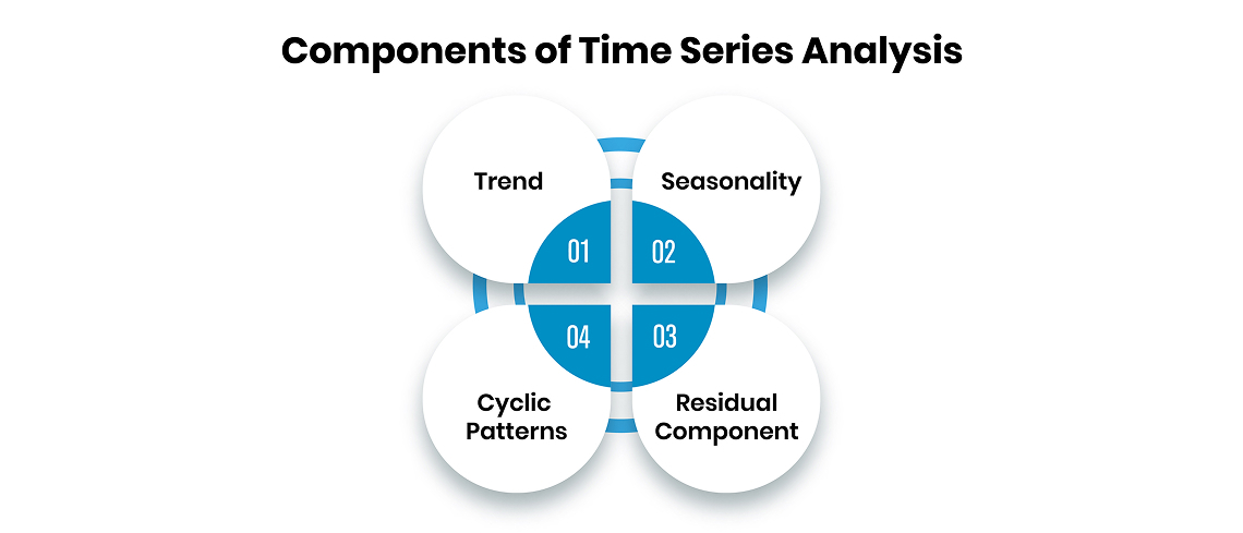
- Trend: A trend is a long-term movement in time series data that moves upwards, downwards, or remains stagnant. It can be either positive or negative, have macroeconomic causes, or be brought about by technological shifts or demographics. Trend analysis is helpful because it allows researchers to establish long-term behavior and comprehend structural changes in data.
- Seasonality: Seasons are cyclical and recurring changes that can occur daily, weekly, monthly, or during other periods of regular recurring occurrence. For retail goods, sales go high during the festive season, while energy consumption varies. Seasonal fact management improves forecasts based on periodic business movements.
- Cyclic patterns: Unlike seasonality, these are not based on the calendar, and their patterns may not repeat after a fixed interval. They arise due to the cyclical nature of economic models, business development life cycles, and other environmental factors. Cyclic behavior typically takes many years and statistical models are used to identify peaks in the data.
- Residual component: This component cannot be accurately predicted by the model as it may be influenced by events that are not always predictable, like natural calamities or political events. Since these values do not have any specific trend, they are termed noise and need to be transformed to enhance the accuracy of future values.
Working with Time Series Data in Python
The preprocessing step for time series analysis involves preparing the data structure to make it easy to model in Python and forecast trends efficiently. The first step is to import some fundamental libraries, including Pandas and Matplotlib, to handle data on time variants. Formatting datetime columns correctly is essential, especially when using an incorrect data type, which can cause various computations.
Critical Stages in the Analysis of Time Series Data:
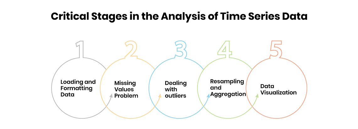
- Loading and Formatting Data: Load datasets using pandas and convert date columns into datetime type indexes that can be easily sliced.
- Missing Values Problem: When working with a time series, gaps, such as weekends, holidays, or system crashes, always occur. Some approaches include forward filling, interpolation, or even rolling average gaps.
- Dealing with outliers: Outliers in the data can create unusual peaks and troughs that distort trends. These approaches are simple and reliable singling out methods, including the IQR or z-score filtering.
- Resampling and Aggregation: Converting time series data into daily, weekly, or monthly data helps analyze long-term value and reduce fluctuations.
- Data Visualization: Line plots, histograms, and seasonal decomposition assist in getting trends, seasonality, and irregular fluctuations before applying the model for the forecast.
Preprocessing the data to be analyzed in time series analysis is crucial to producing the best model and accurate forecasts. Clean data always gives the correct predictions, preventing poor analytics results.
Time Series Data Exploration
Analyzing time series data is an essential step before modeling since it helps identify the trends and characteristics to be expected. Time series analysis in Python can be conducted using various methods, and the data is prepared differently. Here's an overview:
Checking Stationarity:
- Ensure stationarity in most time series models. The null hypothesis of the Augmented Dickey-Fuller (ADF) test determines whether a time series data set is stationary.
- The null hypothesis of the ADF test states that the data has a unit root, meaning it is non-stationary. Therefore, if the p-value is less than 0.05, the data is stationary.
Code Snippet:
from statsmodels.tsa.stattools
import
adfuller
adf_test = adfuller(time_series_data)
print('ADF Statistic:', adf_test[0])
print('p-value:', adf_test[1])
Differencing to Remove Trends and Seasonality:
- Differencing is used to make time-series stationary through the subtraction of prior observations.
- The simplest form of difference is first-order differencing, but higher-order differencing may be required in some instances, such as higher-degree trends.
Code Snippet:
time_series_diff = time_series_data.diff().dropna()
Transformations for Data Normalization:
- Logarithmic Transformation: This transformation is helpful to reduce data variability with high variance.
- Box-Cox Transformation: Another technique used to normalize data spread around the mean besides applying logarithm transformation.
Code Snippet:
import numpy as np
time_series_log = np.log(time_series_data)
Time Series Forecasting Methods
Forecasting in time series analysis involves predicting future values based on previous values observed. Several methods in statistics and machine learning analyze time-dependent data, and each technique captures data characteristics somewhat differently.
- Exponential smoothing: This technique handles discontinuous data while removing short-range fluctuations associated with irregular data collection. Compared to the moving average, exponential smoothing assigns weights to past observations that decrease with time, making it suitable for short-term forecasting.
- Autoregressive Integrated Moving Average (ARIMA): The ARIMA model integrates Autoregressive, Integrated, and Moving averages to deal with trends in sequence data. It is highly used for forecasting time series data, particularly for stationary time series data.
- Power of LSTMs: Long Short-Term Memory (LSTM) is a type of Recurrent Neural Network suitable for inferring long-term dependencies and parameters in a series more suited for non-linear and high-dimension time series forecasting.
Implementing ARIMA for Time Series Forecasting
The Autoregressive Integrated Moving Average (ARIMA) is one of the most efficient techniques for dealing with non-stationary time series data. It consists of three components:
- Autoregression (AR): Captures relationships between an observation and previous time steps.
- Integration (I): Differencing the data to ensure that it has no trend or seasonal parts that would make it non-stationary.
- Moving Average (MA): Models dependencies between observations and residual errors.
Steps to Build an ARIMA Model
1. Identifying p, d, q Parameters
- Use the Augmented Dickey-Fuller (ADF) test to check stationarity.
- Apply differencing (d) if needed to make the series stationary.
- Determine AR (p) and MA (q) orders using Autocorrelation (ACF) and Partial Autocorrelation (PACF) plots.
2. Training and Evaluating the Model
- Fit the ARIMA model on historical data.
- Evaluate the model using metrics like MAE and RMSE.
3. Making Future Predictions
- Generate forecasts for upcoming periods.
- Plot actual vs. predicted values for validation.
Code Snippet for ARIMA Model
import pandas as pd
import numpy as np
import matplotlib.pyplot as plt
from statsmodels.tsa.arima.model import ARIMA
from statsmodels.tsa.stattools import adfuller
# Load dataset
df = pd.read_csv("time_series_data.csv", parse_dates=["Date"], index_col="Date")
# Check stationarity
result = adfuller(df["Value"])
if result[1] > 0.05:
df["Value"] = df["Value"].diff().dropna()
# Fit ARIMA model
model = ARIMA(df["Value"], order=(2,1,2))
model_fit = model.fit()
# Make predictions
forecast = model_fit.forecast(steps=10)
# Plot results
plt.figure(figsize=(10,5))
plt.plot(df.index, df["Value"], label="Actual")
plt.plot(pd.date_range(df.index[-1], periods=10, freq="D"), forecast, label="Forecast", color="red")
plt.legend()
plt.show()
Evaluating Time Series Models
The accuracy of a time series analysis model must always be determined to confirm its ability to produce reasonable predictions in the future. Since time series also include dynamic factors such as trend and seasonality, the correct set of metrics enables the assessment of how well the model captures them. Measures are used to understand the errors within the prediction to enhance forecast precision. Furthermore, back-testing is widely used in the models’ validation procedure, as it involves testing them on historical data before implementation.
- Mean Absolute Error (MAE): This is the most basic and memorable evaluation metric. It measures the deviations of the predicted value from the actual value in terms of the mean magnitude of those errors. A low MAE implies that a model is closer to the exact values, but it does not consider the size of the numbers.
- Root Mean Square Error (RMSE): This metric slightly focuses on more significant errors by squaring them before finding the average. It is useful when a significant error needs to be penalized to identify one that might affect the decisions made.
- Mean Absolute Percentage Error (MAPE): This method also produces errors in absolute terms of actual values, but it is more manageable with large-scale datasets than MAE and RMSE. It is mainly used to evaluate the performance of different models using different time series.
Conclusion
Time series analysis helps forecast by providing periods, seasonal changes, and cyclical patterns. In AI, breaking down these components improves accuracy, besides, reliable preprocessing creates reliability. Using statistical and machine learning models also improves prediction, and assessing the models based on KPIs guarantees their effectiveness. Lastly, for decision-makers who often use data to drive decisions, Python for time series analysis is a skill that cannot be overlooked


