Decision trees are a very popular and important method of Machine Learning (ML) models. The best aspect of it comes from its easy-to-understand visualization and fast deployment into production. To visualize a decision tree it is very essential to understand the concepts related to decision tree algorithm/model so that one can perform well decision tree analysis.
Knowing about the decision trees and the elements of decision tree visualization, will surely help to create and visualize it in a better way. Great decision tree visualization is something that speaks for itself. One must have all the inputs before creating it. It is always advisable to improve the old way of plotting the decision trees so that it can be easily understandable.
Decision Trees
Decision trees are the core building blocks of several advanced algorithms, which include the two most popular machine learning models for structured data - XGBoost and Random Forest. A Decision Tree is a supervised Machine learning algorithm. It is used in both classification and regression algorithms.
The decision tree is like a tree with nodes. The branches are based on a number of factors. It splits data into branches till it accomplishes a threshold value. A decision tree consists of the root nodes, children nodes, and leaf nodes. Each leaf in the decision tree is responsible for creating a specific prediction. A decision tree learns the relationship present in the observations in a training set, which is represented as feature vectors x and target values y, by examining and condensing training data into a binary tree of interior nodes and leaf nodes.
The disadvantage of decision trees is that the split it makes at each node will be optimized for the dataset it is fit to. This splitting process will generalize well to other data. However, one can generate huge numbers of these decision trees, tuned in slightly varied ways, and combine their predictions to create some of the best models.
The visualization decision tree is a tremendous task to learn, understand interpretation and working of the models. One of the biggest benefits of the decision trees is their interpretability — after fitting the model, it is effectively a set of rules that are helpful to predict the target variable. One does not need to be familiar at all with ML techniques to understand what a decision tree is doing. That is the main reason, as it is easy to plot the rules and show them to stakeholders, so they can easily understand the model’s underlying logic.
For instance, find a library that visualizes the decision nodes split up the feature space. It is also uncommon for libraries to support visualizing a certain feature vector as it weaves down through a tree's decision nodes; one could only find one image showing this.
Essential elements of decision tree visualization:
Before digging deeper, it is very essential to know the most important elements that decision tree visualizations must highlight:
- Decision node feature versus target value distributions:
A decision node is where the tree splits according to the value of some attribute/feature of the dataset. One must have an understanding about how separable the target values are depending upon the feature and a split point. - Decision node feature name and feature split value:
A root node is the node where the first split takes place. One must know which feature each decision node is testing and where in that space the nodes splits the observations. - Leaf node purity that affects the prediction confidence:
Leaves with low variance among the target values (regression) or majority target class (classification) are more reliable predictors. - Leaf node prediction value:
Leaf node is the terminal node, which predicts the outcome of the decision tree. There must be an understanding of what is being predicted by the leaf from the collection of target values. - Numbers of samples in decision nodes:
Sometimes they are very helpful to know where most of the samples are being routed through the decision nodes. - Numbers of samples in leaf nodes:
The main objective of a decision tree is to have a larger and purer leaves. Nodes with few samples are possible indications of over fitting. - An understanding of how a particular feature vector is run down the tree to a leaf:
This helps explain why a particular feature vector gets the prediction it does. For instance, in a regression tree predicting apartment rent prices, one might seek a feature vector routed into a high predicted price leaf because of a decision node that checks for more than three bedrooms.
Creating and visualizing decision trees with Python
While creating a decision tree, the key thing is to select the best attribute from the total features list of the dataset for the root node and for sub-nodes. The selection of best attributes is being achieved with the help of a technique known as the Attribute Selection Measure (ASM). By using the ASM one can very quickly and easily select the best features for the respective nodes of the decision tree.
For creating and visualizing decision trees with Python the classic iris dataset will be used. Here is the code which can be used for loading.
- Data: Iris Dataset
import sklearn.datasets as datasets
import pandas as pd
iris=datasets.load_iris()
df=pd.DataFrame(iris.data, columns=iris.feature_names)
y=iris.target
Sklearn will generate a decision tree for the dataset using an optimized version of the Classification And Regression Trees (CART) algorithm while running the following code.
from sklearn.tree import DecisionTreeClassifier
dtree=DecisionTreeClassifier()
dtree.fit(df,y)
One can also import DecisionTreeRegressor from sklearn.tree if they want to use a decision tree to predict a numerical target variable.
- Model: Random Forest Classifier
Here two versions are created-one where the maximum depth is limited to 3 and another where the maximum depth is unlimited. If one wants they can use a single decision tree for this. But here let’s use a random forest for modeling
from sklearn.ensemble import RandomForestClassifier # Limit max depth model = RandomForestClassifier(max_depth = 3, n_estimators=10) # Train model.fit(iris.data, iris.target) # Extract single tree estimator_limited = model.estimators_[5] estimator_limited DecisionTreeClassifier(class_weight=None, criterion='gini', max_depth=3, max_features='auto', max_leaf_nodes=None, min_impurity_decrease=0.0, min_impurity_split=None, min_samples_leaf=1, min_samples_split=2, min_weight_fraction_leaf=0.0, presort=False, random_state=1538259045, splitter='best') # No max depth model = RandomForestClassifier(max_depth = None, n_estimators=10) model.fit(iris.data, iris.target) estimator_nonlimited = model.estimators_[5] - Creation of visualization
Now that the creation of decision tree is done, let’s use the pydotplus package to create visualization for it. One needs to install pydotplus and graphviz. Thses can be installed with the package manager.
Graphviz is a tool that is used for drawing graphics; it takes help from dot files. Pydotplus is a module to graphviz’s dot language. Here is the code:
from sklearn.externals.six import StringIO
from IPython.display import Image
from sklearn.tree import export_graphviz
import pydotplus

dot_data = StringIO()
export_graphviz(dtree, out_file=dot_data,
                filled=True, rounded=True,
                special_characters=True)

graph = pydotplus.graph_from_dot_data(dot_data.getvalue())
Image(graph.create_png())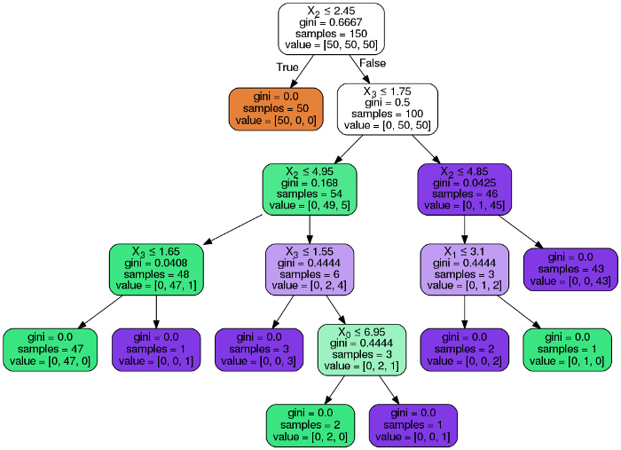
The ‘value’ row in each node gives details related to the many observations that were sorted into that node, which fall into each of the categories. The feature X2, which is the petal length, was able to completely distinguish one species of flower (Iris-Setosa) from the rest.
Conclusion
Visualizing a single decision tree can help provide an idea of how an entire random forest makes predictions: it's not random, but rather an ordered logical sequence of steps. The plots created using this library are much easier to understand for people who do not work with ML on a daily basis and these plots can help in conveying the model’s logic to the stakeholders.
Industrial data science is about building a smarter company infrastructure. It should blur or thin the line between the operational and digital processes. Big data analytics provides innovative opportunities to establish an efficient process, reduce cost and risk, improve safety measures, maintain regulatory compliance, and better decision-making.


