


Data preparation is an essential first step in any data science or machine learning project. Real-world data is often incomplete, inconsistent and lacking in certain properties that make it unsuitable for modeling. Pandas library for data manipulation are required to handle missing values, outliers, data types etc. and transform the raw data into a clean and optimized form for modeling.
Python is becoming increasingly popular for data science and analysis due to the powerful open-source libraries available for working with data like Pandas. Pandas is a Python library that supports working with labeled/relational or sequentially-indexed data in various formats like NumPy, lists, JSON, CSV, databases etc. It provides high-performance, user-friendly data structures and data analysis tools to make working with structured/tabular data intuitive. The core data structure of Pandas is DataFrame, which acts like a spreadsheet, allowing labeling of axes (rows and columns), selection of slices, and efficient arithmetic operations on data.
This article demonstrates useful techniques in Pandas to perform common data wrangling tasks like filtering, transformations, imputing missing values, merging etc. These data manipulation techniques in Pandas will help efficiently prepare any dataset for modeling using basic Pandas functions.
Importance of Data Manipulation
Data manipulation is a crucial skill for any data analyst or scientist. Mastering techniques for cleaning, transforming and restructuring data allows analysts to prepare it for effective analysis that produces reliable insights. Without proper manipulation, data issues could introduce errors or hide important patterns, undermining results.
Pandas represents data as labeled columns within DataFrame objects, allowing data to be organized and accessed like a SQL table. This tabular structure streamlines common manipulation tasks.
Booleans and indexing enable straightforward filtering of DataFrames. Boolean conditions can select subsets of data based on multiple-column criteria. Methods like .loc[] and .iloc[] subsetting allow precise slicing of data. These aids expedite extracting relevant portions of data for focused analysis.
Transforming data types and imputing missing values prepares them for modeling. Functions such as .astype(), .replace() and .fillna() homogenize variable formats and complete records. This cleaning fortifies data integrity prior to statistical examination or neural network training.
Reshaping extends the usefulness of data. Wide-format DataFrames become long to simplify time series or plot grouping. Pivoting rotates aggregated records for exploratory analysis. Hierarchical indexes grant multidimensional views of information. These shape modifications broaden analyzable patterns within data.
Data provenance and versioning prevent surprises from outdated analysis. Merging joins supplementary records while preserving origins. Copying isolates modified DataFrames to test changes safely. Resetting reverts modifications for refreshed evaluation. Jointly, these revision controls secure the reproducibility of insights.
Visual inspection reveals issues too subtle for formulas. Plots uncover outliers, distributions, relationships and more with just a few lines of code. This visual verification aids decision-making all through the data preparation cycle.
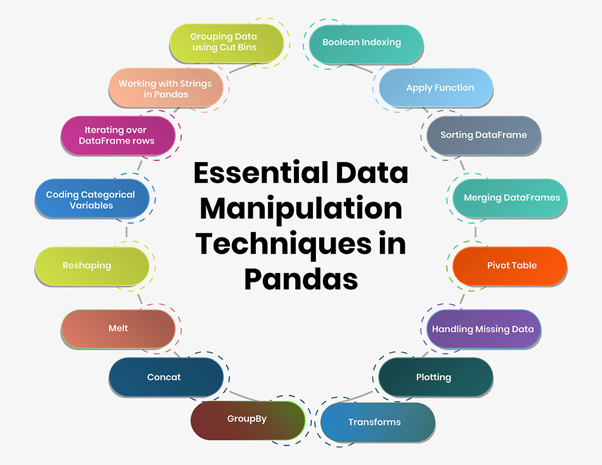
Essential Data Manipulation Techniques in Pandas
The following are some essential techniques in Pandas:
1. Boolean Indexing
Boolean indexing in Pandas allows filtering DataFrame rows or columns based on a conditional criterion. It is useful when you need to extract specific subsets of data based on conditions.
For example, to extract rows where 'Gender' is 'Female' and 'Education' is 'Not Graduate':
import pandas as pd
data = pd.read_csv('data.csv')
filtered_data = data[(data['Gender']=='Female') & (data['Education']=='Not Graduate')]
This returns a new DataFrame with only rows satisfying both conditions. Multiple conditions can be chained using the & (AND) and | (OR) operators.
2. Apply Function
Pandas apply() method applies a function along one axis of the DataFrame and returns the transformed values. This is useful for column-wise or row-wise operations on DataFrame.
For example, to count missing values in each column:
def missing_count(col):
return col.isnull().sum()
missing_counts = data.apply(missing_count, axis=0)
A lambda function or custom-defined function can be passed to apply(). This is handy for feature transformations directly on DataFrame.
3. Sorting DataFrame
Sorting DataFrame based on values allows ordering or ranking data. The Pandas .sort_values() method can sort on multiple columns.
For example, to sort DataFrame by 'ApplicantIncome' and 'CoapplicantIncome' in descending order:
sorted_data = data.sort_values(['ApplicantIncome','CoapplicantIncome'], ascending=False)
The index is also maintained during sorting. Additional parameters like ignore_index, kind etc. provide control over sorting.
4. Merging DataFrames
Merging or joining DataFrames is essential when data is present in multiple files that need to be combined. Pandas .merge() does this seamlessly for labeled data.
For example, to merge property rates DataFrame with main data based on 'Property_Area':
rates_data = pd.DataFrame({'rates':[1000,5000,12000]},index=['Rural','Semiurban','Urban'])
merged_data = data.merge(rates_data, left_on='Property_Area', right_index=True)
Different merge types and parameters prevent unwanted joins. This is key for integrating multisource data.
5. Pivot Table
Pivot tables allow aggregating and restructuring data to get insights. Pandas .pivot_table() creates pivot tables to summarize and manipulate data easily.
For example, to count loan applications by gender and city:
pt = data.pivot_table(index=['Gender','City'], values='Loan_ID',aggfunc='count')
This pivots the DataFrame to count Loan_IDs for unique combinations of gender and city. Aggregate functions like mean, sum, and std can also be applied.
6. Handling Missing Data
Real-world data often has missing values. Filling or imputing these is important for modeling. Pandas offers multiple methods to handle missing data:
- Fill NA's with a value using .fillna()
- Impute missing values per column using median, mean etc.
- Drop rows/columns with missing values using .dropna()
For example, to impute missing 'Gender' values with the mode:
from scipy import stats
mode = data['Gender'].mode()[0]
data['Gender'] = data['Gender'].fillna(mode)
Different approaches suit different missing patterns. Appropriate handling reduces bias in modeling.
7. Plotting
Visualization helps understand data better. Pandas integrates well with Matplotlib to easily plot DataFrames.
For example, to plot a histogram of 'ApplicantIncome' by 'Loan_Status':
import matplotlib.pyplot as plt
data.groupby('Loan_Status')['ApplicantIncome'].plot(kind='hist')
plt.show()
This gives intuitions on distribution and outliers. Both one-dimensional and two-dimensional plots are supported.
8. Transforms
Feature transforms help extract better information from raw features for modeling. Pandas UDFs allow transforming DataFrames using custom functions.
For example, to bin numeric 'ApplicantIncome' into categorical bins:
bins = [0, 20000, 40000, 60000, np.inf]
labels = ['Low','Medium','High']
data['IncomeLevel'] = pd.cut(data['ApplicantIncome'],bins,labels=labels)
New features like interactions, changes of scales etc. can be added. This enriches the feature space.
9. GroupBy
Grouping allows aggregate analysis on DataFrame partitions. Pandas .groupby() splits data into groups based on some criteria and performs operations on these groups.
For example, to find the mean loan amount by education:
data.groupby('Education')['LoanAmount'].mean()
This groups DataFrame by 'Education' and computes the mean of 'LoanAmount' for each unique education level. Multiple grouping criteria and aggregate functions can be specified.
10. Concat
Concatenating DataFrames comes up frequently while working with multiple heterogeneous datasets. Pandas .concat() helps concatenate/merge DataFrames vertically (row-wise).
For example:
df1 = pd.DataFrame({'A':[1,2],'B':[3,4]})
df2 = pd.DataFrame({'A':[5,6]})
merged_df = pd.concat([df1,df2])
Parameters control the axis and joining behavior. This is useful for batch/parallel data processing where separate chunks need combining.
11. Melt
Melt is the opposite of pivot/pivot_table. It is used to convert multiple column values into row values with an identifier column. This is useful to transform wide skinny DataFrames into long tall structures.
For example:
name_vars = ['Subject', 'Test']
value_vars = ['Score1','Score2']
melted_df = pd.melt(data, id_vars=name_vars, value_vars=value_vars)
Converts columns to row values for easier modeling of multiple measures for each subject/test.
12. Reshaping
Reshaping changes the DataFrame shape by stacking/unstacking levels of columns or indexes. Pandas stack() and unstack() methods do this reshaping along axis levels.
For example:
data = pd.DataFrame({'Param1': [1,2],
'Param2': [3,4]},
index=['Obs1', 'Obs2'])
reshaped = data.stack()
This stacks columns with a new level index. Overall reshaping helps convert data between wide-long formats suiting modeling approaches.
13. Coding Categorical Variables
Converting categorical strings to integer codes for modeling is important. We can define a generic function:
def coding(col, codeDict):
colCoded = pd.Series(col, copy=True)
for key, value in codeDict.items():
colCoded.replace(key, value, inplace=True)
return colCoded
And apply it as:
data["Loan_Status_Coded"] = coding(data["Loan_Status"], {'N':0,'Y':1})
This technique prepares clean coded data for modeling.
14. Iterating over DataFrame rows
To iterate and apply logic row-wise, we can do:
for i, row in data.iterrows():
# row is a Series
if(row['column'] == 'condition'):
row['new_column'] = 'value'
This allows validating/modifying data row-by-row when needed rather than bulk operations.
15. Working with Strings in Pandas
Pandas has methods to handle string columns to clean up, parse, and split data using regex.
We use the following methods to process name columns:
data['Name'] = data['Name'].str.title() # Title case standardization
data['Initials'] = data['Name'].str.extract('([A-Za-z]+)\.') # Extract initials
replace(), contains(), startswith() etc are other useful string methods.
16. Grouping Data using Cut Bins
Grouping continuous numerical variables into logical bins often provides more intuitive insights compared to raw values. Using cut(), we can bin the 'ApplicantIncome' into slabs as:
data['IncomeGroup'] = pd.cut(data['ApplicantIncome'],bins=[0,25000,50000,75000,100000],labels=['Low','Medium','High','Very High'])
Now aggregation can be done based on these bins rather than raw values.
Conclusion
This article covered useful Pandas techniques that form the core of data manipulation tasks in Python. Effective feature engineering using these techniques prepares untidy raw data into a clean optimized form for modeling.
These were some useful techniques in Pandas for working with datasets. Choose the right techniques as per your requirement to efficiently extract insights from data.